Lab 3: Baby Names

Each year after the Census Bureau releases its list of the names given to the babies born in the most recent year, it is common for the press to release a series of stories on baby names or trends in baby names. It has also recently become a popular data set for teaching introductory data science. In fact, one year after I created the original version of this lab in 2016, a babynames package was introduced to R which has the data pre-loaded for you. However, it is good practice for us to try loading these files on our own.

This lab is meant for you to practice using R. You must submit it, but sample solutions will be provided on the second day of the lab, so completing and submitting the lab should be straightforward. You should focus in this lab on becoming more comfortable with R.

Data Downloads:

For this lab, you will need to download and unzip a file containing the Census Bureau baby names data.

Data Description

The data set is a zipped folder of .csv text files that contains the Census Bureau counts of names of baby boys and girls born each year from 1880 to 2014. These data include any name-gender combination for which there were at least five babies born in that year. There is a separate text file for each year from 1880 to 2014. For example, the file named yob1942.txt contains the counts of names for all boy and girl babies born in 1942.

Each row in a text file is of the format [name, gender, count]. For instance, some sample lines in the text file yob1942.text might be:

• Mary, F, 7312

• John, M, 6400

The first line would indicate that 7,312 girls born in 1942 were given the name Mary. This lab asks you to use these data, along with R, to analyze how naming patterns in America have changed over the last 150 years.

Remember to keep all of your work in R-notebooks or R-scripts and to save frequently! NOTE: Many of the steps below can be combined, but I have tried to write them out to make them more clear, and I have tried to rely only on "core" R functions, which is what we have covered so far in class. There are also multiple ways to complete most of these objectives. Feel free to experiment with others.

Objective 1. Load the data files into an R data frame

• Before you begin: Although the data are available from 1880 to 2014, it may take a long time for your laptop to load in the data for all of these years! I recommend starting with a more recent window – say, from 1970 to 2014 – or if that still takes more than a few minutes, an even more recent window. However, those of you with more powerful laptops may be able to handle the entire data set, and I have made all of the files available because it is interesting to see how baby naming patterns in the US were different before the numerous waves of immigration that changed US demographics during the twentieth century.

• The data must first be read into a data frame in RStudio. The most efficient way to do this is to use a for loop to loop through all of the text files in the folder, read each into RStudio, and as you read each of them in, add them to a data frame. This is easiest if executed and tested in a series of steps. Note, although the steps are outlined below, the actual code for this Objective is provided for you after the steps are described.
  • Download and unzip the Census Bureau files, set your working directory to the folder where you have downloaded these files and use the read.csv() command to try reading a single .csv file into RStudio and assigning it to an object name. Check that it works as expected by examining the created object in RStudio.
  • Create a data frame called babynames and set it to NULL.

    babynames = NULL

  • Create a vector containing the numbers 1880 through 2014 (or whichever years you have chosen), which are the years that you will need to loop through to read all of the files in the folder.
  • Create a for loop that iterates through the values in the year vector from 1880 to 2014. As mentioned in class, there are very few reasons to use a for loop in R, but for our purposes it is clear in this context, you can use a function called lapply to skip the for loop.
  • Put the read.csv() command into the for loop. Use text string concatenation to create an appropriate file name to pass to the read.csv() command in each iteration of the loop.
  • The contents of each read.csv() command should be passed to a temporary data frame. To this temporary data frame, you should add a new column that contains the year of the file from which the data is drawn from (for all rows in the data frame). Then, $rbind$ the temporary data frame containing only the contents of the most recent file + the new column with the year of that file to the data frame babynames which contains the running total contents of all the files you have read up until that point.
  • After the for loop is created, babynames should contain the data from all files, and each row should have an additional column containing the year of the file that the data came from. If you are using all the years from 1880 to 2014, you should end up with 1,825,433 rows. After you have completed the steps above, assign sensible column names to your data frame using the names command in R.

To get you started quickly, I have provided the code to load in the files. If this works and makes sense, you can begin with Objective 2.

Set your working directory to the folder where the name files are located on YOUR computer.

setwd("~/Dropbox/Teaching/oidd245/labs/baby/data/")

Because we are going to append rows to this dataframe, we need to start with an empty initial dataframe.

babynames = NULL

For loop to read in the file and append it to a “running total dataframe” called babynames. If loading in the data set is taking too long, you may want to change 1950 to something more recent.

for (year in (1970:2014)) { foo = read.csv(paste("yob", toString(year), ".txt", sep=''), header=FALSE) babynames = rbind(babynames, cbind(foo, year)) }

• NOTE: If you have never written a for loop before, or are new to programming, this first step can easily take a large portion of the first class day (and yet only produce a few lines of code), and that is okay! It is worth spending time on this to understand how it is working, and after this step is completed, the rest of the lab goes more quickly. If it is still not clear to you what is happening in the for loop, you can find a more thorough explanation here.

Objective 2. Plot how the popularity of your own name has been changing over the years

You should now have available in your RStudio environment a data frame containing the counts of all name-gender combinations in each year from your beginning start year to 2014.

• Plot how the number of people in the data set that share your name and your gender varies from year to year. If your name does not appear in the data, use the name of a lab partner (or choose your favorite)!

• To complete this objective, first create a new data frame myname that contains only the rows from babynames that match both your name and gender (use the which command in R to do this). Then, from myname, plot counts against years for the data, and don't forget to label the axes and give a sensible title to your plot.

Objective 3. Visualize the growth in girl names from 1880-2014

Create a plot of the number of different baby girl names in each year from 1880 (or whatever you have chosen as the initial year in your data set) to 2014. Plot the number of different names there are for girls reported by the Census Bureau in the data each year. In other words, no matter how many girls have a given name, it should only count as one name.

• First, create a data frame that only includes baby girl names for each year.

• Then, the table command is a useful way to compute the number of names for each year in your data frame.

• Plot the results.

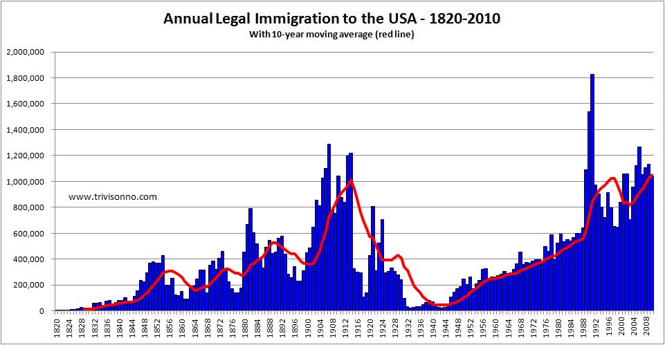
It may be interesting to visually compare the results with the following image.

Objective 4. Write a function to generate the most popular names for a given gender and year

Write a function toptennames that takes two arguments, gender and year, and returns the top ten names for that gender in that year. This function should:

• Create a new data frame ttn containing only rows that match on gender and year.

• Use the order command to reorder ttn so that it is decreasing by counts.

• Return the top ten rows of the reordered data frame.

After running your function, test it by calling it on girl names for the first and last years that appear in your data set:\

> print(toptennames(1880, "F")) > print(toptennames(2014, "F"))

Objective 5. Compute the most gender-neutral names

Generate a list of the ten names that, in 2014, were relatively popular for both baby boys and baby girls. To do this, use the following condition: for names for which there are at least 1000 people in the year with that name (including boys or girls), compute the difference between boys and girls with the name. Then, we will call those names with the smallest magnitude difference between the two the most “gender neutral” names. This is not the best definition of gender-neutral, but it is a definition and is straightforward to implement.

To complete this objective:

• Keep only rows from 2014.

• Create a data frame male with only boy names and their counts.

• Create a separate data frame female with only girl names and their counts.

• Merge the two data frames on name.

• Keep only those rows where the sum of counts for boys and girls is at least 1000.

• Compute the absolute value of the difference between counts of boys with the name and counts of girls with the name.

• Use sort or order to sort the data frame by the absolute value you just computed.

• Use head to find the top ten gender neutral names.

Objective 6. Convert your code into Python

Ask ChatGPT to take the code you developed for Objective 1 — including setting your directory path to the proper place and running through the for loop — and convert it into Python. Then, put it in a Python script file in RStudio as will be demonstrated in class, and test the output to ensure that it works. You can check the length of a list in Python using the len() command.

Now, for fun (!), use ChatGPT to convert your code into Julia and into Scala, which are other popular data science languages (but there is no need to test if they work).

• How do you think the emergence of large-language models like ChatGPT will impact the demand for what we refer to as “coding” skills?

• As these tools become increasingly widespread, which skills do you think will become less valued in the technical community and which skills will become more valued?

EXTRA CREDIT.

Now, turning back to R, attempt to “prompt engineer” ChatGPT to aid you in creating the R-based solutions for Objectives 1 through 5 above from scratch (i.e. without asking it to convert existing code). For credit, provide screenshots of the prompts you use and the R-based output it generates, and demonstrate that the code — or an edited version of it — works.

• When creating code from scratch in this way, which tasks become faster?

• On which tasks do you find yourself spending time instead?